The Molecular Stimulator
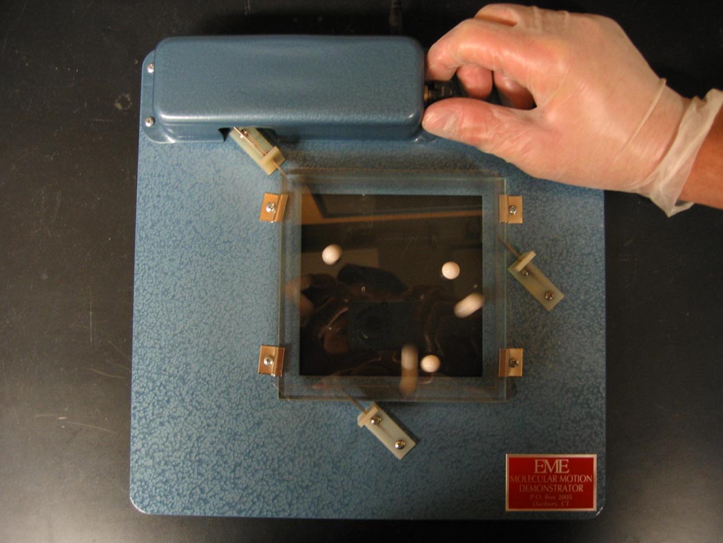
Small plastic balls jostled about provide a realistic simulation of the "molecular dynamics" of atoms in a gas.
Ingredients: molecular simulator
Procedure: A complete recipe follows.
1. Add plastic balls to achieve desired gas "density."
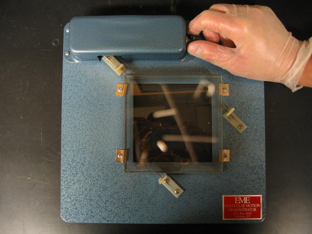
2. Adjust rate of frame oscillation to achieve desired "temperature."
Understanding:
In the demonstration, the motion of the plastic balls provides a relatively faithful "molecular dynamics" simulation of a rare gas, such as argon. When atoms of argon are separated by a few atomic diameters, they attract each other through a relatively weak soft dispersion attraction. At short distances, the atoms "overlap" and there is a strong repulsion between the atoms.
At sufficiently high temperatures, the energy in the kinetic motion of the argon atoms is much greater than the attractive energy between the atoms. The attractions become insignificant, and the atoms of argon interact like "hard spheres" feeling only repulsive interactions during collisions. That dynamics of "hard spheres" is captured by the molecular simulator in the dynamics of the plastic "atoms."
The microscopic kinetic molecular theory of gases tells us that atoms and molecules in a gas are moving with a variety of speeds. Suppose we could enter a balloon of a simple atomic gas, and carefully observe the motion of the atoms. If we recorded the speed of each passing atom, made many observations, and then plotted that data, we would find a distribution of speeds. We would find very few atoms moving very slowly, and very few atoms moving very quickly. Most of the atoms would move with a speed close to the average speed, uave.
That distribution of speeds is known as the Maxwell distribution. Why does it have the form that it does? We can think of our gas as having a fixed number of atoms. The total amount of energy in the gas is also fixed.
If we think of our simple gas as an ideal gas, the energy of an atom of mass m moving with speed u is its kinetic energy
Eatom = mu2/2
It turns out that if we randomly distributed a fixed amount of energy among the atoms, we can expect that the probability of finding an atom with a certain amount of energy will decrease exponentially with increasing energy. The details are interesting.
The resulting probability distribution is
probability(Eatom) = kBT exp[-Eatom/kBT]
probability(u) = 4 π (m/2 π kBT)3/2 u2 exp[-mu2/2kBT]
ump = (2kBT/m)1/2
Notice that the distribution is skewed. More atoms will be found moving with a speed that is higher than the most probable speed, rather than slower than the most probable speed. That makes the average speed
uave = (8kBT/πm)1/2
The first "molecular dynamics" simulations of liquids and gases were carried out on a computer in the late 1950's by Bernie Alder and his coworkers. As a model of the atoms they used "hard spheres" - spheres that interacted only through repulsions, like tiny pool balls. They found that their simulations could provide a reasonably faithful simulation of real liquids and gases at many densities and temperatures.
Our molecular simulation using plastic balls is a similarly faithful representation of the molecular dynamics of a gas. By adjusting the rate of motion of the oscillating frame, the average speed of the balls can be increased, raising the "temperature" of the gas.
In a simulation of a cold gas, the plastic balls move at an average speed of 6 cm/s. What is the average speed of the simulated "cold" argon gas, in m/s? What is the temperature of the simulated "cold" argon gas, in K?
In a simulation of a hot gas, the plastic balls move at an average speed of 1 m/s. What is the average speed of the simulated "hot" argon gas, in m/s? What is the temperature of the simulated "hot" argon gas, in K?
You can check your answers here.
Interpreting the molecular simulation at the atomic scale
Question:
Suppose we had ten plastic balls, each one-half centimeter in diameter, placed in a cubic box ten centimeters on a side. Imagine that the box of plastic balls is a simulated gas of argon atoms. Take the diameter of an argon atom to be 3.1 Å. What is the mass density of the gas, in g/L? Compare your result to the mass density of argon gas at STP.