|
This page summarizes
detector tests and characteristics. At present, there are two summaries,
reflecting the major detector operating changes instituted during the
Nov/Dec 2005 detector tuning run. Future continued tuning of the detector,
and commissioning of new operating modes is planned. As these occur, new
values for detector characteristics will be added to this page.
- For
data obtained after 12/1/2005
- For
data obtained before 12/1/2005
For Data
Obtained since 12/1/2005
Conversion Gain:
~8.21 e/ADU (2006/06/27 - dpc)
Read Noise:
17.8 e/read (2006/06/27 - dpc)
Well Depth:
about 7,500 ADU (this is about the lowest seen on the detector)
Dark Current:
~10 e/s/pixel (but not linear with time)
Operating Temperature:
33.5K (currently set to 35K)
Linearity Correction:
4th order
|
|
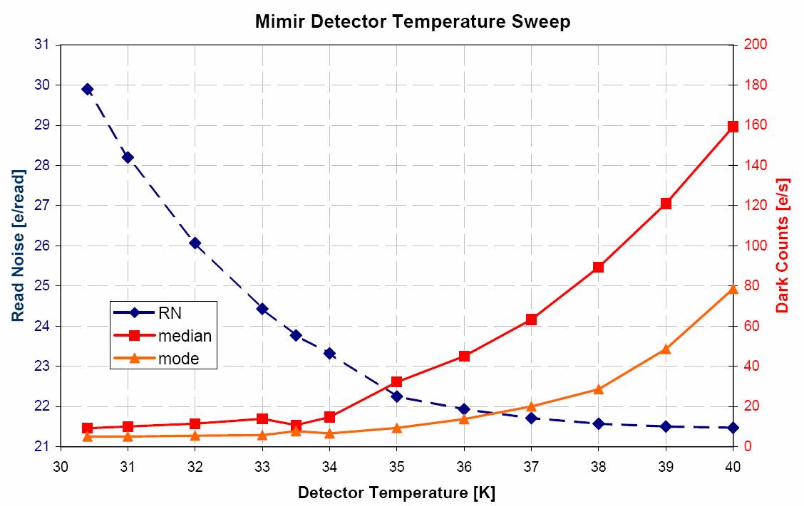
Plot of Read Noise and Dark Current versus
Detector Temperature. The strong rise in dark current beyond 34K,
but the continuously decreasing read noise with temperature led us
to set the detector temperature at 33.5K. Click on the image to see
the full sized version of the plot. |
|
|
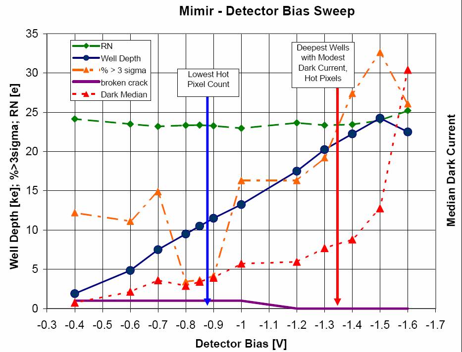
Plot of pixel well depth, dark current, and read noise
versus detector bias. Until 12/2005, we had been operating with about
0.6V of reverse bias, not much above starvation. Two new operating
points were identified, corresponding to the blue and red vertical
arrows. The blue arrow, with bias of 0.875V has the lowest dark current
and hot pixel count and well depth of about 11-12,000 ADU. This is
the ideal operating point for most JHK imaging and spectroscopy. A
second operating point, at a bias of 1.35V has even deeper pixel wells,
nearly 22,000 ADU, but much higher dark current and hot pixel counts.
This mode could be employed for LM imaging and LM spectroscopy, where
the shorter integration times are able to offset the dark current
and hot pixel problems. Click on the image to see the full sized version
of the plot. |
For Data
Obtained prior to 12/1/2005
Detector Conversion
Gain
A series of multiple
exposures in the dome flat-field screeen were obtained for a range of
integration times, with and without the flat screen illuminator lights
on. All images were linearity-corrected. Difference and sum images were
created at each integration time and the results plotted as variance
of the differenced images versus mean counts in the summed images. The
data were linearly fit for each quadrant, yielding a mean conversion
gain (inverse of the slope term) of 9.7 electrons per analog to
digital unit (ADU) (for the 20050605 and 20050615 data sets,
and a somewhat higher 10.3 value for the 20050517 data set, obtained
before a detector operating voltage change).
Detector Read Noise
From the y-intercept
of the conversion gain plot, adjusted for the contributions from the
eight readouts (four each for each of the two images differenced), the
rms value for one read, averaged over the four quadrants, was found
to be 21.1 electrons per pixel (20050605 & 20050615,
for the 20050517 data the value is 23.8 electrons per read).
Detector Pixel Well
Depth
In the mean vs variance
plot, the variance deviates beyond some point, signaling that many of
the pixels had reached saturation. The saturation value depends on quadrant
and even/odd row, which is embodied in one of the the linearity correction
images. Here, the quadrant averaged value was found to be 30,200
electrons (20050605 & 20050615, and 31,500 for 20050517).
Detector Dark Current
At a detector temperature
of 30 K, the measured dark current is about 1 ADU/s/pixel, or roughly
10 electrons per second per pixel, though this varies
with exposure time (there is a "prompt" dark current contribution
that decays with time). Observers are urged to obtain darks with exposure
times identical to their science images, rather than scaling from long
darks.
Linearity Correction
InSb arrays are
inherently non-linear in their response to light. Mimir data are corrected
for this effect via application of a linearity correction algorithm,
applied on a pixel-by-pixel basis. The data used to calculate the corrections
are drawn from the same detector calibration data described above. The
form of the correction is a quartic correction, applied after correcting
both first and second reads back to the plateau (reset release) time
for each exposure.
Additional, extensive
testing of pixel timing and detector operation was performed during Engineering
Run #3 at the Perkins telescope:
Detector (pixel)
Timing Diagrams
Aug
2004 (initial timing)
Dec 2004 - three
different pixel timing models: "Working" (HTML,
Excel);
"Trophy" (HTML,
Excel);
"Dream" (HTML,
Excel)
AladdinIIIwaveforms.s
timing files: "Working" (?) (txt)
Detector Temperature
Sweep
The detector temperature
was varied from about 20 K to 40 K and bias frames taken to measure
read noise and dark current versus temperature. We found the expected
rise in read noise for the lower temperatures and the rise in dark
current for the high detector temperatures. There appears to be a
region from about 30-34 K where the read noise is stable and the dark
current is low. We also noted that the ghosting increased dramatically
as the temperature was lowered, implying that operating at the warm
end of the acceptable region might further reduce ghosting or permit
faster pixel read times. (Excel
file).
 Thumb
of Detector Heater Power vs Detector Temperature - click to see full
plot Thumb
of Detector Heater Power vs Detector Temperature - click to see full
plot
 Thumb
of Read Noise and Dark Current vs Detector Temperature - click to
see full plot Thumb
of Read Noise and Dark Current vs Detector Temperature - click to
see full plot
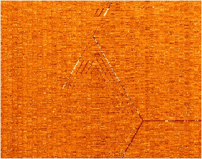
 Thumb
of portion of an image showing increased ghosting of the crack at
low detector temperatures (this image was when the detector was at
24 K) - click to see full size plot Thumb
of portion of an image showing increased ghosting of the crack at
low detector temperatures (this image was when the detector was at
24 K) - click to see full size plot
Pixel Integration
Time Sweep
The ARC A/D boards
have, as part of their video signal processing chain, an integrator
circuit. This test was designed to find the minimum integration time
needed to achieve low-noise operation. Because the coversion gain
depends linearly on this pixel integration time, the read noise measured
in these short bias frames was divided by the pixel integration time
to yield the dependent figure of merit plotted along the Y-axis versus
the pixel integration time (X-axis). Clicking on the thumbnail image
below brings up the full plot, which shows a "knee" at about
600 ns. The polynomial fit has no physical meaning but conveys some
of the sense of the drop in RN from low integration times to a plateau
beyond 600 ns. (Excel
file)
 Thumb
of pixel integration time plot - click to see full plot Thumb
of pixel integration time plot - click to see full plot
|